

Using Convolutional Neural Networks to Identify Fish Species in Camera Footage
I participated in my first Kaggle challenge a few months ago. For a PhD level course I took in Computing and Software (CAS 771), Introduction to Big Data Systems we had to choose a term project that showcased Big Data.
Vague, I know.
I decided to take the opportunity to learn about multilayer neural networks (commonly known as a multilayer perceptron, or MLP) and convolutional neural networks (CNNs).
I built my own Ubuntu computer for this contest. Well mostly for the contest, I was quite computer limited only using a Surface Pro 3 (integregrated graphics card...). My father helped me assemble the PC since he's pretty tech savvy and we made a day of it. Its rocking a GTX 1060 with 6 gigs of video card RAM and a total of 1280 CUDA cores. I got the latest graphics card driver, CUDA 8.0, CuDNN 5.1, Tensorflow and Keras. I was ready for action.
The Contest
The Kaggle Nature Conservatory Fisheries Monitoring classification competition consists of classifying the species of fish found in security camera footage. Successful classifiers for the competition need to be robust to a variety of conditions such as: day, night, rain, multiple image resolutions and multiple magnifications. We propose a method herein using an ensemble of pre-trained (Inception V3) convolutional neural networks (CNNs) which have been previously trained using the ImageNet image library. The models will be fine-tuned, starting with ImageNet weights, using the fisheries training data and a variety of tools such as: stochastic gradient descent, dropout, batch-normalization, weight decay, and data augmentation.
Illegal fishing and overfishing are quickly becoming a massive global problem as fish stocks have declined over the past century. To tackle this problem, organizations such as The Nature Conservatory of California have proposed methods to track the amount of fish being caught. Methods such as human observers on boats and cameras have both been explored, with the former being resource intensive and the latter being an incredibly large big data challenge.
On November 14 2016 a contest was launched through the data-science competition website Kaggle called The Nature Conservatory Fisheries Monitoring [1]. The challenge proposed is to create an algorithm that can identify the species of fish in camera footage. The idea is that if cameras can snapshot images periodically, a supervised machine learning framework can parse through the pictures and record what types of fishes are being caught by each boat. As an incentive for contest participants, The Nature Conservatory of California raised $150,000 in venture capital funds to use as prize money for the top 5 ranked teams.
A dataset of 3777 images with eight labeled classes was given for the competition. The evaluation criteria is given by a multi-class logarithmic loss function

Background
Convolutional Neural Networks (CNNs) have been a disruptive emerging innovation in the image recognition world recently. Alex Krizhevsky, Ilya Sutskever, and Geoffrey E. Hinton won the 2010 ImageNet competition using CNNs [2]. The 2015 ImageNet was won by employees at Google and their Inception architecture is what is used for the present study [3]. All current competitors in ImageNet today do indeed use some form of a CNN.
In another more recent Kaggle contest launched by NOAA, the challenge involved identifying the species of whales taken from satellite images and the winning team also used CNNs for feature mapping [4]. CNNs are a variant of a multilayer neural network (also known as a multilayer perceptron, or MLP). CNNs have additional layers prior to the dense neuron layers of a traditional MLP which are used to create discriminating features in an image for classification.
An MLP consists of:
- An input layer of one node per input parameter
- A set of hidden layers which may consist of multiple layers of multiple nodes
- The output nodes which in the case of classification will consist of one output node per class
- An arrow is drawn between every input node, hidden layer node, and output node which represents the weight or the strength of the connection between the nodes
Every hidden layer node contains a transfer function or activation function, . Where is the weighted sum of the input nodes multiplied by each respective weight. This is outlined in the figure below.
With the number of hidden nodes and the number of layers of hidden nodes typically constrained, the degrees of freedom in the MLP are the values of the weights. By using training data (input data with known classes), the values of the weights in the network are tuned to produce the correct output class.

Bias terms are ignored in the above cartoon for the sake of simplicity
Weights are optimized to reduce the error between the calculated values and the target (expected) values. The error is optimized via gradient descent and back-propagating the error to update the values of the weights. A scalar factor is applied to this gradient known as the learning rate which dictates how large of a jump is made per optimization cycle on the error surface.
Generally each optimization cycle can be performed after each training observation (on-line), but this is computationally expensive. On the other hand, performing gradient descent after using all training observations will result in very slow convergence. A compromise known as a mini-batch is typically used where a small random sample of the observations is typically used and gradient descent is performed after each of these batches to find the optimum value of each weight.
The MLP is straightforward for cases of regression and classification when using small sets of numerical input parameters. In the case of image processing and image recognition however, it is clear that some pre-processing step is required to reduce the amount of data contained in the image. For a 3 colour channel RGB image that has a resolution of 1920 x 1080 pixels, the amount of input parameters contained in the image is over 6 000 000. To produce a successful classification, this will require a large multilayer neural network and a large training set to tune the network. For image processing, a successful preprocessing step before being inputted into the fully connected MLP is to perform a series of convolutions and image pooling steps. This is the basis of the CNN.
Convolution layers in the CNN will take the input image and convolve the image with a kernel window of a specified size. In the case of the 3 x 3 kernel, it can be thought of as choosing a pixel in the image, and looking at all of its nearest neighbor pixels (producing a 3 x 3 window centered on the chosen pixel). This ‘patch’ is multiplied with the kernel matrix and divided by the total number of pixels in the patch to produce one value on a new image at the location of the chosen pixel from the first image. Depending on what the values are inside the kernel window, various transformations can be applied to the image such as blurs, and edge sharpening. The image is then typically down-sampled using a process called pooling. In the case of max-pooling, the image is max-binned in 2 dimensions to produce an image with half of the size as the original.
By combining many layers of convolutions and pooling, the final image “features” can then be flattened into a vector which becomes the input parameters into a dense neural network (MLP). The final layer of the MLP outputs to a soft-max classifier which puts a probability to a potential classification.
Transfer Learning (Inception V3 trained on ImageNet)
Using Keras and Tensorflow the Inception V3 model [3] can be loaded with its dense layer removed (it outputs to 1000 classes for the ImageNet competition). The final pooling layer is then connected to a new MLP and a softmax classifier. There is a stark improvement in the speed of network training by using a pre-trained network (such as the Inception V3 architecture with the ImageNet weights) when compared with a randomly initialized network [4].

Using Inception V3 on All Classes
Using a train-validation split of 80/20, all eight fish classes were randomly sampled (stratified class sampling). Using the Inception V3 architecture, the class probability of each image was determined after training using a softmax classifier. The original Inception V3 MLP was removed and replaced with a 512 neuron layer and an 8 neuron layer outputting to the softmax classifier.
A stochastic gradient descent approach was used with weight decay to fine-tune the model over 80 epochs. Using Nesterov momentum (momentum = 0.9), constant learning rates (1e-5), and weight decay (equal to the learning rate over the number of epochs) the modeled converged by the end of the calculation. The total amount of tunable parameters exceeded 55 000 000. Images were resized to 299 x 299 image before being inputted into the network in batches of 16. Data augmentation was performed to increase the number of images that the model sees. This includes rotations, translations, normalizations, and flips. The results of the convergence are shown below in Figure 4.
The loss criterion used is categorical cross-entropy and it was found that the training accuracy exceeded 80 % with the validation accuracy being over 90 %. The reason why the validation accuracy was higher than the training accuracy is due to over-fitting measures such as dropout being present in the training data. The total training time was about 3 minutes per epoch, which amounts to 3 to 4 hours of training time.

Pipeline Inception V3 Models
To improve validation accuracy over 90 %, it is clear that a different approach will need to be used. Fine-tuning the network by adding new data augmentation, or growing the MLP layers was found to only marginally improve results (< 2% increase in accuracy). The new approach is two-fold. First, one Inception V3 classifier is used for binary fish – no fish classification. Then, the seven fish classes are inputted into a new Inception V3 classifier for species identification. The methodology is showed in Figure 5.

The purpose of splitting up the classes is to reduce the amount of variance that each CNN sees in its dataset. An eight class classification is more difficult to resolve than a seven class classification. In addition to this, the NoF class has many of the same features as each fish species (boat, water, people etc.).
A drawback of creating a binary Fish – No Fish classifier is the small amount of training data of the ‘NoF’ class (465 images) when compared with ‘Fish’ (3312 images). To circumvent this problem, each NoF image was cropped into four quadrants and added to the original images to produce an augmented dataset containing 2325 NoF images. Since the Inception V3 classifier resizes the images to 299x299, each 1920x1080 image can be cropped without losing significant detail. An example of the nature of the cropping is shown in Figure 6.
Using the 2325 NoF and 3312 Fish images, the dataset was divided into an 80/20 train-validation split with stratified class sampling. With the original ImageNet MLP removed, the Inception V3 convolutional layers were added to an MLP containing a layer of 1024 neurons, 1024 neurons, then to a 2 neuron layer which outputs to a softmax classifier.

Model training took place over 100 epochs with 8 images per mini-batch. Using a stochastic gradient descent method (Nesterov momentum = 0.9, learning rate = 1e-4), categorical cross-entropy was minimized by updating the values of the weights in the network. Batch-normalization was used for image normalization, while dropout (0.5) and weight decay (1e-6) was used to mitigate overfitting. The training time was 3 – 4 minutes per epoch which amounts to 5 – 6 hours total. The convergence of class accuracy and categorical cross entropy over the amount of epochs is shown in Figure 7. Various hyperparameters were tweaked such as: learning rate, number of epochs, the number of MLP layers, and the amount of neurons per layer. The model parameters discussed above and shown in Figure 7 had the best results with ~97 % class accuracy.

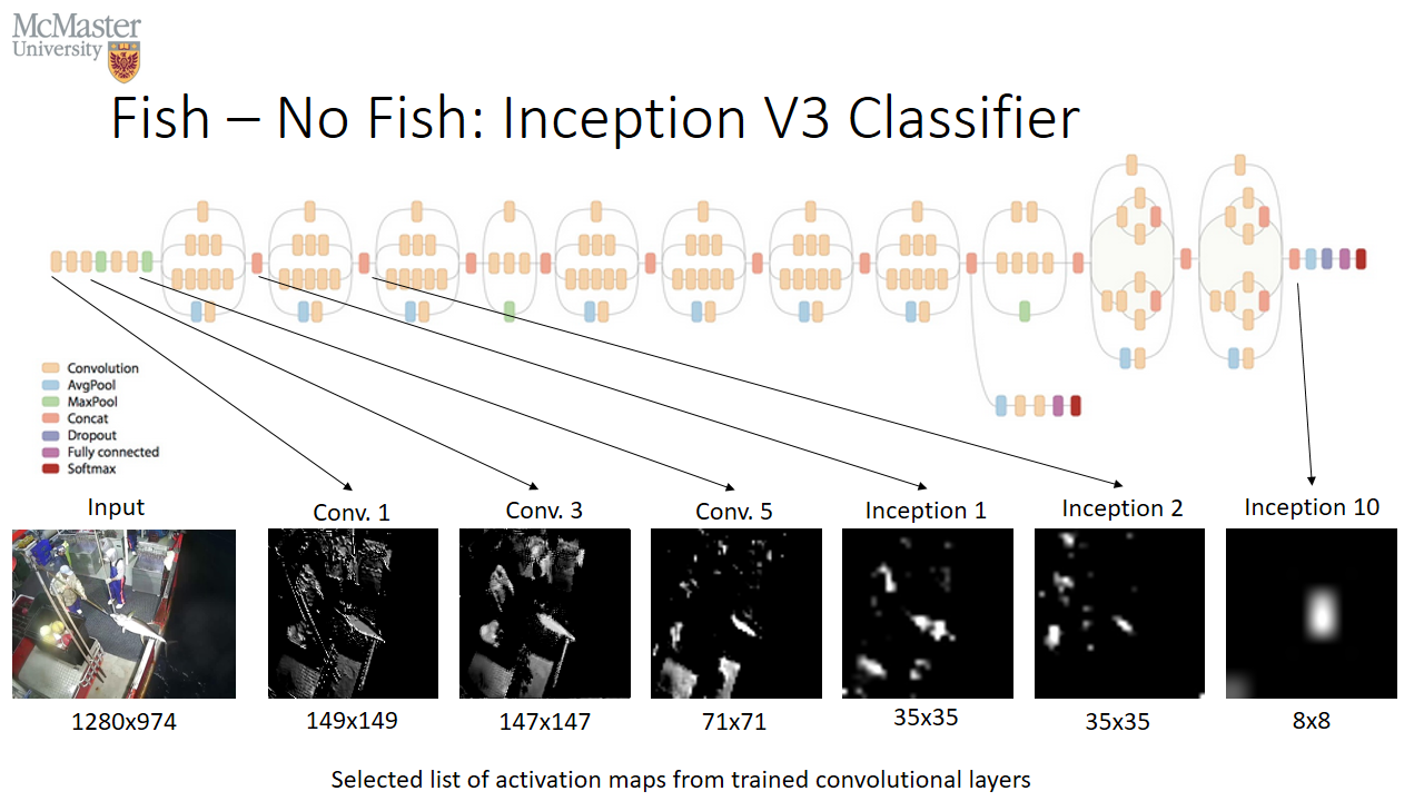
After training the Fish-NoF classifier, the activations of each convolution layer were visualized to better characterize the success of the model training. It was found that the first few convolution layers would do image transformations such as edge highlighting. Later filters would select specific objects in the activation map. By the final inception layer (Inception Layer 10), specific pixels were identified which corresponded to the fish. The results of the activation mapping are shown in Figure 8.
The maps shown in Figure 8 were carefully selected to suit the narrative of fish localization. Nearly all trained filters were not relevant to finding the fish and were other features of the image such as fishermen, fishing poles, railings, harpoons and crates. The final Inception 10 concatenation layer contains thousands of filters with only a handful of relevant fish localization filters.
With the class NoF being removed from the rest of the classification (Figure 5), the remaining seven classes were classified using a different Inception V3 classifier (pre-loading the ImageNet weights like in the first classifier). The original ImageNet Inception V3 MLP was removed and the flattened feature vector was connected to three layers of 1024 neuron dense layers and finally to a seven neuron softmax classifier. Between every layer in the MLP, batch-normalization was performed for normalization and a 50 % neuron dropout was used to mitigate overfitting.
Training of this 157 000 000 parameter model took place over 200 epochs with 8 images per batch. Weights were optimized via stochastic gradient descent using a fixed learning rate of 1e-4. Weight decay was set to the learning rate over the total number of epochs. Model convergence is shown in Figure 9. Data augmentation using the Keras Image Generator was used with the same parameters as the binary Fish-NoF classifier. The best validation class accuracy was 97.4 % using the aforementioned hyperparameters.
After approximately 125 epochs the model started overfitting as shown by the arrow in Figure 9. By this point, the validation classification accuracy flat-lined with minimal change over the remaining epochs, whereas the training accuracy and log-loss improved. When the cross-entropy loss of the validation set exceeds the cross-entropy loss of the training set, then we know that gradient descent is optimizing the weights of neurons that are not helpful for the validation set and useful only on images the model has seen before (ie. the training set). The model will quickly diverge from being able a generalizable model, that is – a model that can accurately classify unknown data, to one that can narrowly classify only the data it has previously seen before.

Concluding Remarks
Many tools were effective at improving classification accuracy such as: data augmentation, overfitting tools and convergence tools. Data augmentation using image crops as well as traditional data augmentation (zooms, rotations, flips, shears etc.) was extremely effective at improving accuracy. Dropout, weight decay and batch normalization were all effective at improving convergence and decreasing overfitting.
Pre-trained CNNs were found to be critical in training large generalizable models with over 157 000 000 trainable parameters using a single GPU. Model training is typically hardware constrained and by exploiting the parallel computing capabilities of CUDA-enabled NVIDIA GPUs, a single NVIDIA GTX 1060 was capable of handling this real world problem of identifying small objects in camera footage.
The final classification accuracy of the fish species classifier before overfitting was 97.4 %. Combined with the binary fish – no fish classifier with 98.0 % classification accuracy, the ensemble of CNNs performed significantly better than the single eight class classifier (90 %).
References
[1] https://www.kaggle.com/c/the-nature-conservancy-fisheries-monitoring
[2] Krizhevsky, Alex, Ilya Sutskever, and Geoffrey E. Hinton. "NIPS Proceedings." ImageNet Classification with Deep Convolutional Neural Networks. 2012.
[3] Szegedy, Christian, Wei Liu, Yangqing Jia, Pierre Sermanet, Scott Reed, Dragomir Anguelov, Dumitru Erhan, Vincent Vanhoucke, and Andrew Rabinovich. "Going Deeper with Convolutions." [1409.4842] Going Deeper with Convolutions. N.p., 17 Sept. 2014. Web. 17 Apr. 2017.
[4] http://blog.kaggle.com/2016/01/29/noaa-right-whale-recognition-winners-interview-1st-place-deepsense-io/
[5] https://blog.keras.io/building-powerful-image-classification-models-using-very-little-data.html
[6] Szegedy, Christian, Vincent Vanhoucke, Sergey Ioffe, Jon Shlens, and Zbigniew Wojna. "Rethinking the Inception Architecture for Computer Vision." 2016 IEEE Conference on Computer Vision and Pattern Recognition (CVPR) (2016): n. pag. 11 Dec. 2015. Web. 18 Feb. 2017.


