Unsupervised Learning for Signal Unmixing in Hyperspectroscopy

Background

Hyperspectroscopy is the field of fusing spatial and spectral information together to create powerful chemical maps.

Maps taken from satellites are more often than not hyperspectral. Not only can they produce an image of the X-Y plane below them (the intricacies of thickness and a Z-direction is a topic for another day), but they can capture information in the infrared usually or some other band. This allows an entire spectrum to be captured per pixel and this spatial-spectral fusion in an image is commonly called a spectrum image.

Getting away from satellite images, this is not what I focus on in my Masters. Instead I look at thin (~50 nm) slices of material and shoot an electron beam at them. Per pixel of the x-y plane, I can collect an entire spectrum similar to the way satellites do it. The approach is a little different through. A satellite uses photons, it captures things in the infrared or ultraviolet or whatever wavelength it may be. The things I am imaging are too small for photons to be useful anymore, so we have to switch to something different, electrons.

But hang on, this cannot possibly work. If photons are used the traditional way like in satellites, and they promote ground state electrons in what is being imaged, the object that they are imaging then go back to ground state after excitation producing a characteristic photon describing the transition energy required for electron excitation. If we are using electrons in an electron microscope, what exactly do we measure on the other side? Its not like electrons will promote electrons. We are not measuring photons on the other side either.

So what are we doing here in electron hyperspectroscopy? We shoot electrons through our thin materials, and we recall some grade-school physics related to momentum and scattering. Things can either scatter elastically or inelastically.  Elastically would be like two billiard balls being shot at each other and bouncing away as a result. Inelastically on the other hand is like two vehicles colliding and getting stuck together, energy is used up on the interaction between the bodies. In the elastic case, energy is conserved (the same before and after collision).

When we shoot our electron beam through our material, some electrons scatter elastically and others scatter inelastically. We collect the inelastic electrons on the other side of the material, and since we know the amount of energy the electron started with, and what it left the material with, we can infer some characterizing information about the atom(s) it collided with. This is electron energy-loss spectroscopy.

So whats the problem?

As I briefly touched on earlier in the example with the satellite, thickness and a z-direction is a problem. What we measure in all hyperspectroscopy is a 2D projection of whatever we are looking at. The spectral information we measure per pixel, is actually the entire thickness of that pixel. A problem can arise in the following case:

Okay lets get some of the jargon out of the way in the above slide.

The rectangular prism above in red and green is a sliver of a metal. The best way to think about it is the following: imagine you're doing renovations and contractors just laid down new tile and grout in your bathroom. You want to figure out if they did a good job laying the tile and grout, so you take a small saw and you cut out a piece of the tile and grout at its interface such that you have tile/grout/tile similar to what is shown above with the grain/grain boundary/grain. In the bathroom tile example, we can turn the sample on its side and see its cross section. We can observe if the grout is crisply perpendicular to the tile or if it was laid at an angle. Now imagine you cannot turn the sample on its side (because its something like 100-1000x smaller than a human hair...). How do you know if the boundary you are looking at is on an angle or not through the thickness of the sample?

STEM pixel. The STEM pixel is the Scanning Transmission Electron Microscopy pixel, its what we measure and we have spectroscopic data per one of these pixels.

FIB Lamellae thickness. A Focused Ion Beam lamellae is jargon for a sample cut using an ion beam. In the bathroom tile example, our sample was created by sawing out a rectangular prism from the tile and grout. At the nanoscale, we "saw" out materials by milling into the material with ion beams.

Okay all of this is great. So what is the problem? Well, lets say we want to image that above sample. We want to figure out what the red material is and what the green material is. But in order to do this we need each isolated signal. Are we able to recover the signal of the red material and the green material independently? Will we always have a mixture of the signals at pixels where there is overlap through the thickness of it?

Data Exploration

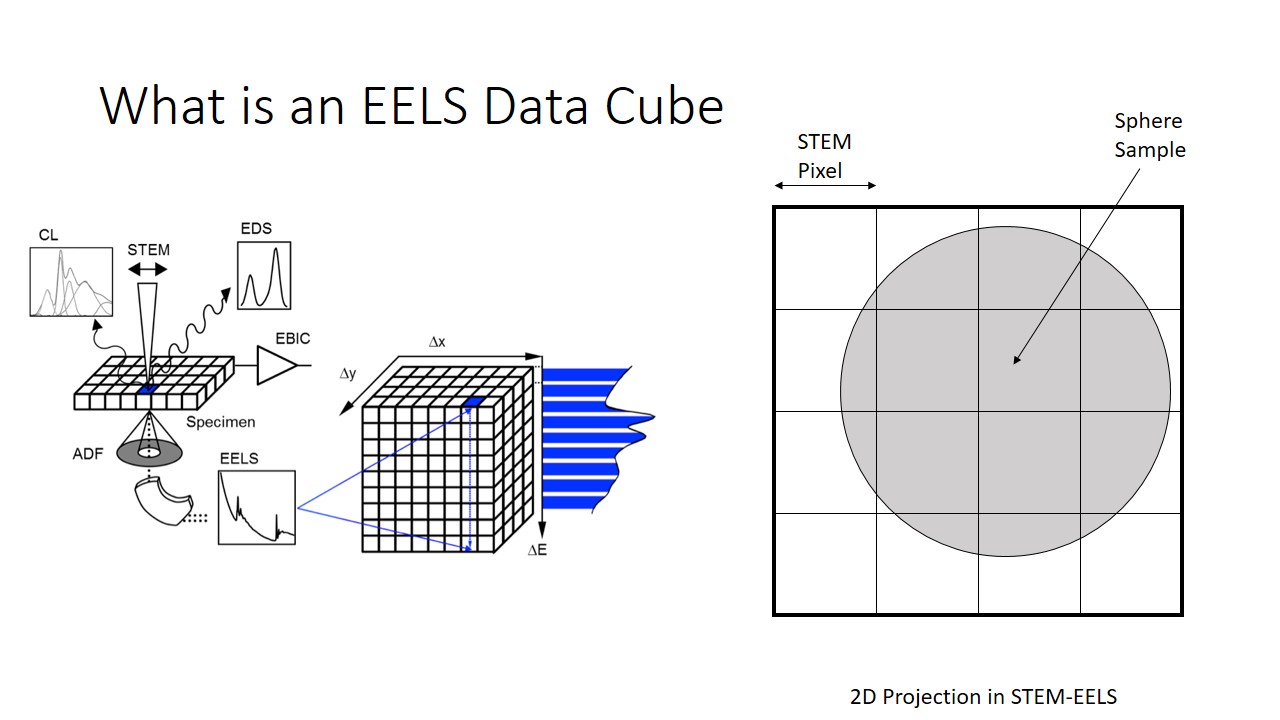
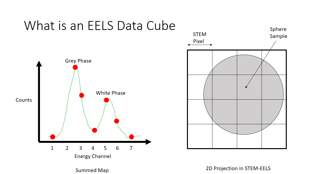
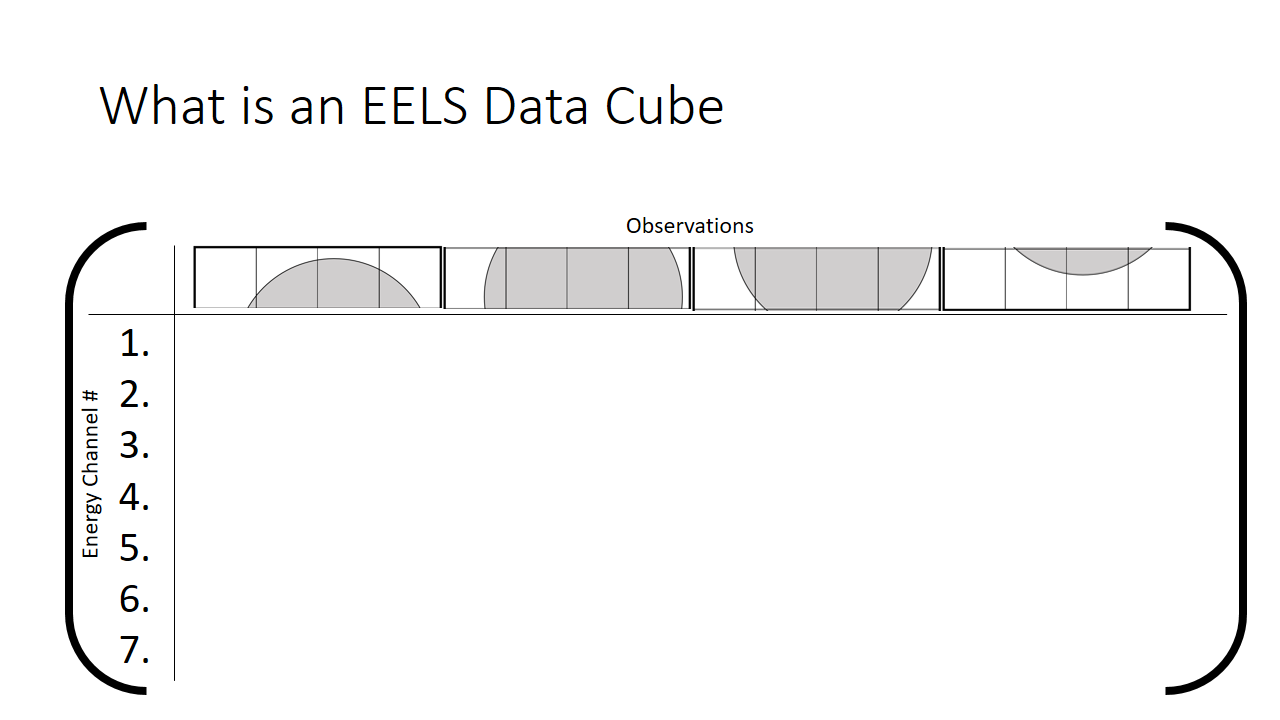
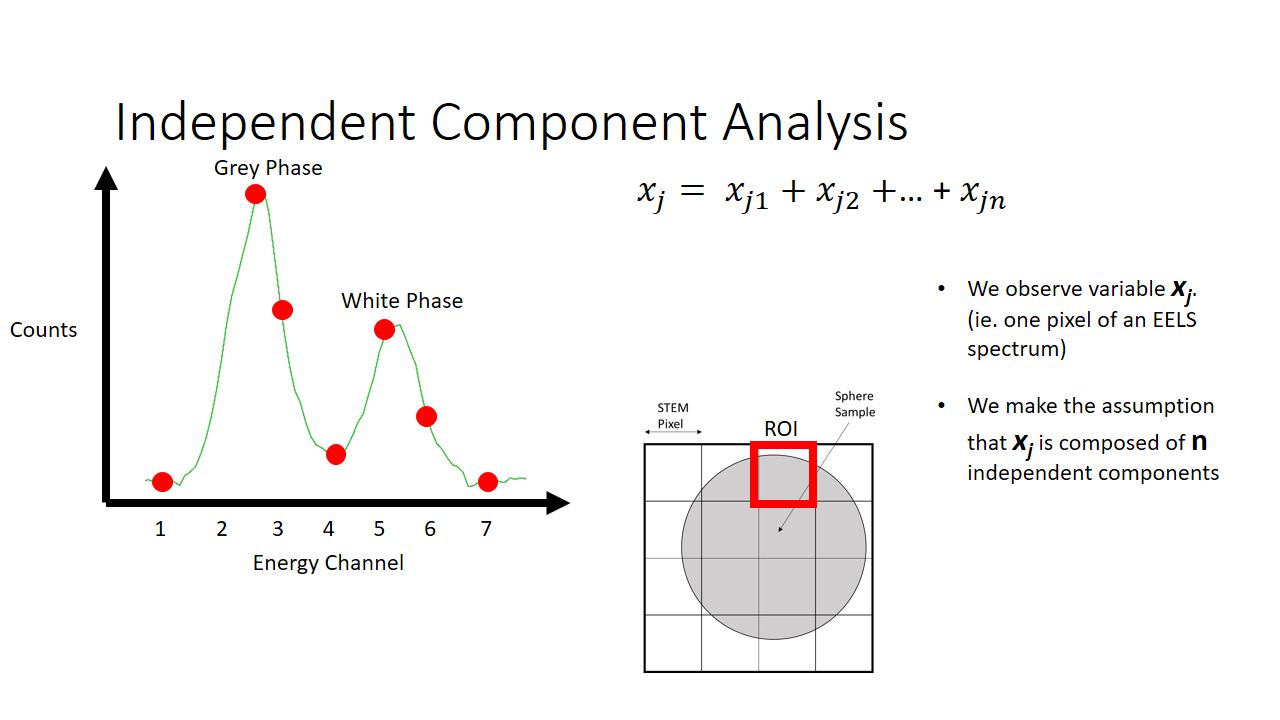
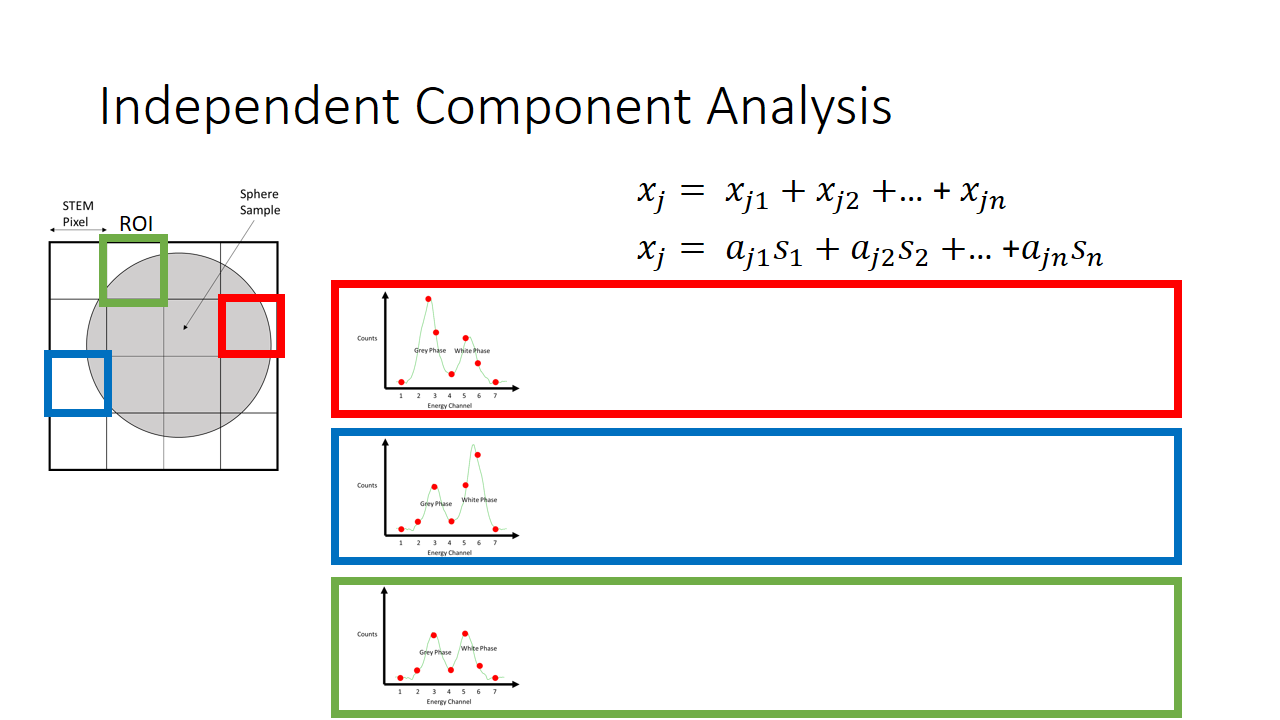
Lets say we are imaging a sphere (above slide). The image we take will be a 4x4 pixel image and we produce a 2D projection of the sphere. The diagram on the left shows the information we have. Per x and y pixel we have an entire histogram of information related to its electron energy-loss spectrum.

I'm not going to make this complicated, so lets imagine we can capture energy information across around 7 bins. You can imagine equivalently a satellite capable of measuring the different colours of the visible spectrum (red, blue, green, etc.).

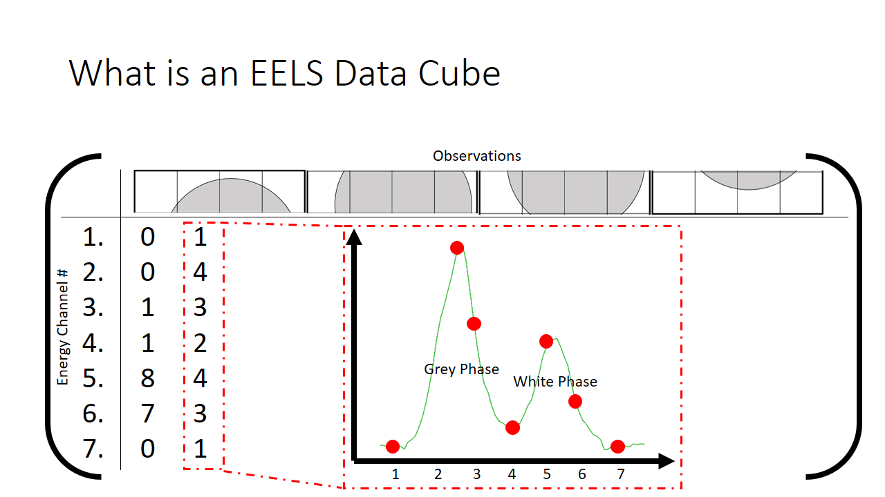
As an example of a spectrum this is what we would get below if we were to sum the histograms of all 16 (4x4) pixels. We see there are more counts of the grey phase (the sphere) and less counts of the white phase (the background, or the substrate that the sphere is on for imaging).

We can rewrite this information into a different notation. A matrix, which is just a series of rows and columns. Each column heading is the location of the pixel, and each row is the bin (the x-axis on the graph shown above, or equivalenty the "colour".)

How we then populate this matrix is shown below. The distribution of the mix of grey and white is shown at each pixel.

The finished matrix is below.

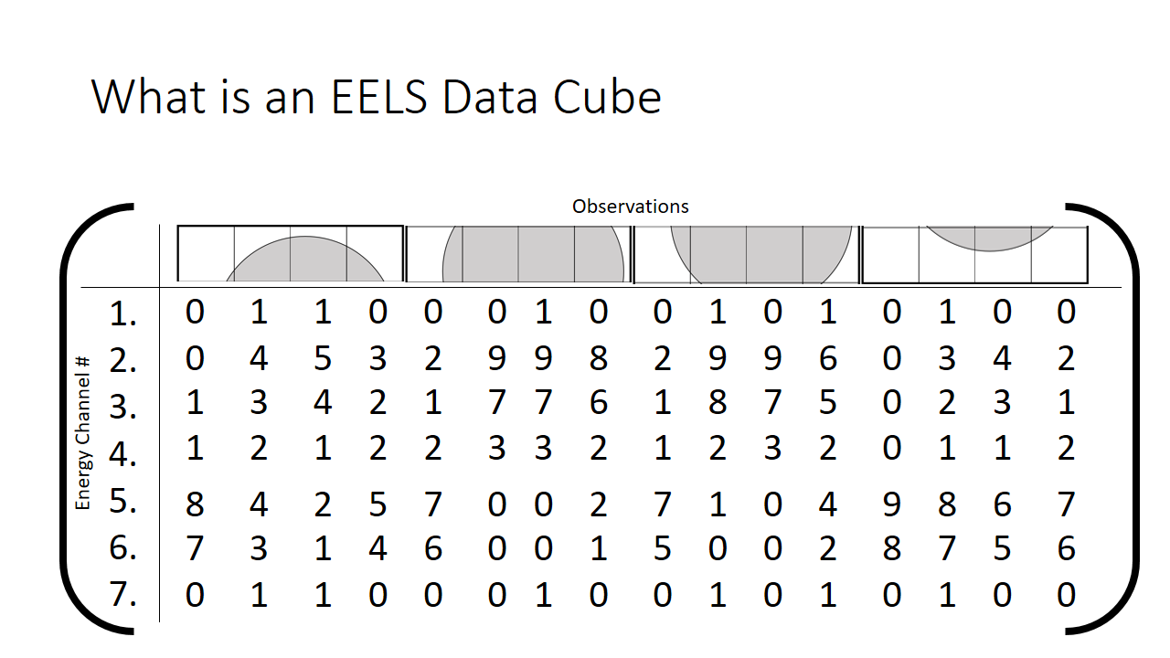
The observant student will notice that there are patterns in the data already. I sort of spoiled that the first hump in the graph is the grey phase, and the second hump is the white phase. What if that fact was not known? One would purely need to use these correlations to deduce what is present in the image. The trends that we can see qualitatively by looking at this matrix I highlight in grey below. They correspond to pixels that are just about purely grey with little mixing.

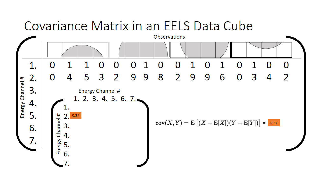
Let us plot just two energy channels across all of our observations (each pixel in the 16 pixel spectrum image we are going to call an observation). We can see as we tweak the value of energy channel 1, the value of energy channel 2 barely budges. This is a qualitative result however, is there any way we can put a number on it? This is precisely what the covariance is used for. It helps us put a number on correlated two features are.

Pre-Processing and Data Cleaning

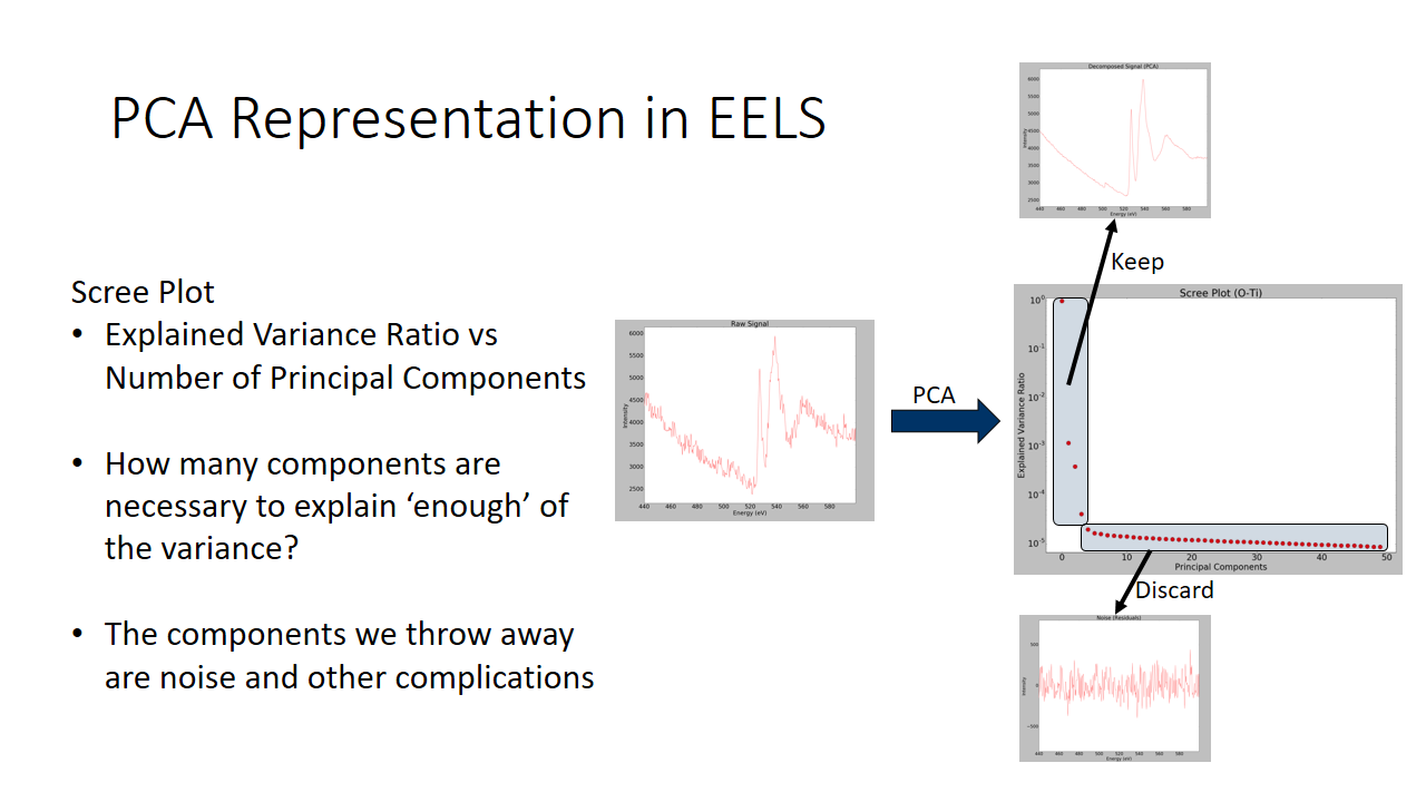
Before we can separate the grey from the white phase, we need to clean the data as much as possible. The approach will be two-fold. First, Principal Components Analysis (PCA) will be used to remove noise and low variance components from the dataset. Next, Independent Component Analysis will be used to isolate the grey from white signals.

Lets first tackle PCA

When we compute the covariance between those two energy channels, we can tuck the result away in the matrix. It will be a symmetric features x features (7x7 in our case for each energy channel) length matrix, our aptly termed covariance matrix.

With this unyieldly matrix (trust me it gets unyieldy when we go to the real size 2048x2048 usually) we can perform another computation, a decomposition of the covariance matrix into its eigenvalues and eigenvectors. This is getting pretty mathy now so I'm not going to explain eigenvalues or eigenvectors too much. It is a mathematical trick (most scientists and engineers hit the "eigendecomposition" function in whatever library they are using) to get us what we want: the directions of largest spread in our data.

Getting the so called "directions of largest spread" is counter-intuitive and confusing. How is this helpful at all? Aren't we trying to remove noise? Why do we keep high variance components and remove low variance components? These are all valid concerns. I will do my best to explain why exactly it is beneficial to remove low variance components and reproject our data along the directions of largest spread.

Look at the figure above on the right. We can see across two dimensions (say height vs mass of adults for example) that there is a clear trend. As variable 1 increases, variable 2 increases. If we were to draw direction vectors on this data, and reproject our data onto those axes, we would have the figure on the right. Zero centered and we can clearly see a direction to the data. It is very easy to see this magic direction vector that "points" in the direction of the main trend when there is two dimensions and the trend is strong. How about when there is 2048x2048 dimensions? Wouldn't it be great if we could calculate numerically what these directions are? This is what the eigenvector is when we decompose our covariance matrix.

As an aside, we will calculate the direction of largest spread (the first eigenvector), then every eigenvector afterwards will be orthogonal to the first and all others. So the 2nd eigenvector is not technically the 2nd largest possible direction of largest spread, but one that is also constrained to being perpendicular to the first.

Still a bit confused? Take a look at the graph below. We will see the raw EELS signal of an oxygen EELS spectra, and we will separate components that explain very little of the variance and keep the directions of largest spread. We can see we adequately denoise the data!

Step 2: Separating Independent Components

We will next delve into the second half of this post, the signal unmixing portion. You may think PCA will sufficiently remove two signals (like the grain vs grain boundary signal) but it cannot. The accuracy is very low and I simply use it as a preprocessing step.

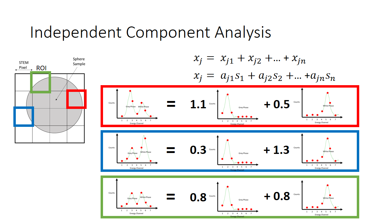
We will delve into another unsupervised method, ICA. ICA is a powerful tool for separating non-gaussian signals from each other. The premise of ICA can be described by the following toy problem.

Cocktail Party Problem. Imagine you are at a cocktail party. There are many people talking at different locations in the room. There are many people listening at different parts of the room. The people listening at different locations in the room thus hear a mixture of the people talking, and it is linearly scaled based off of the distance between the speaker and the listener. How can the listener recover the voices of the original speakers? This is shown schematically in the figure below.

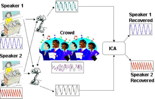
Taken from: http://iiis.tsinghua.edu.cn/~jianli/courses/ATCS2016spring/ATCS-21.jpg

That is a fairly simple toy problem, but how does this apply at all to EELS signal mixing? Well we are going to say that each pixel is like a microphone, or a listener at a party. It will record some linear mixture of the original signal. The original signal here is either the white or the grey phase. In machine learning lingo, each pixel here we term as an observation.

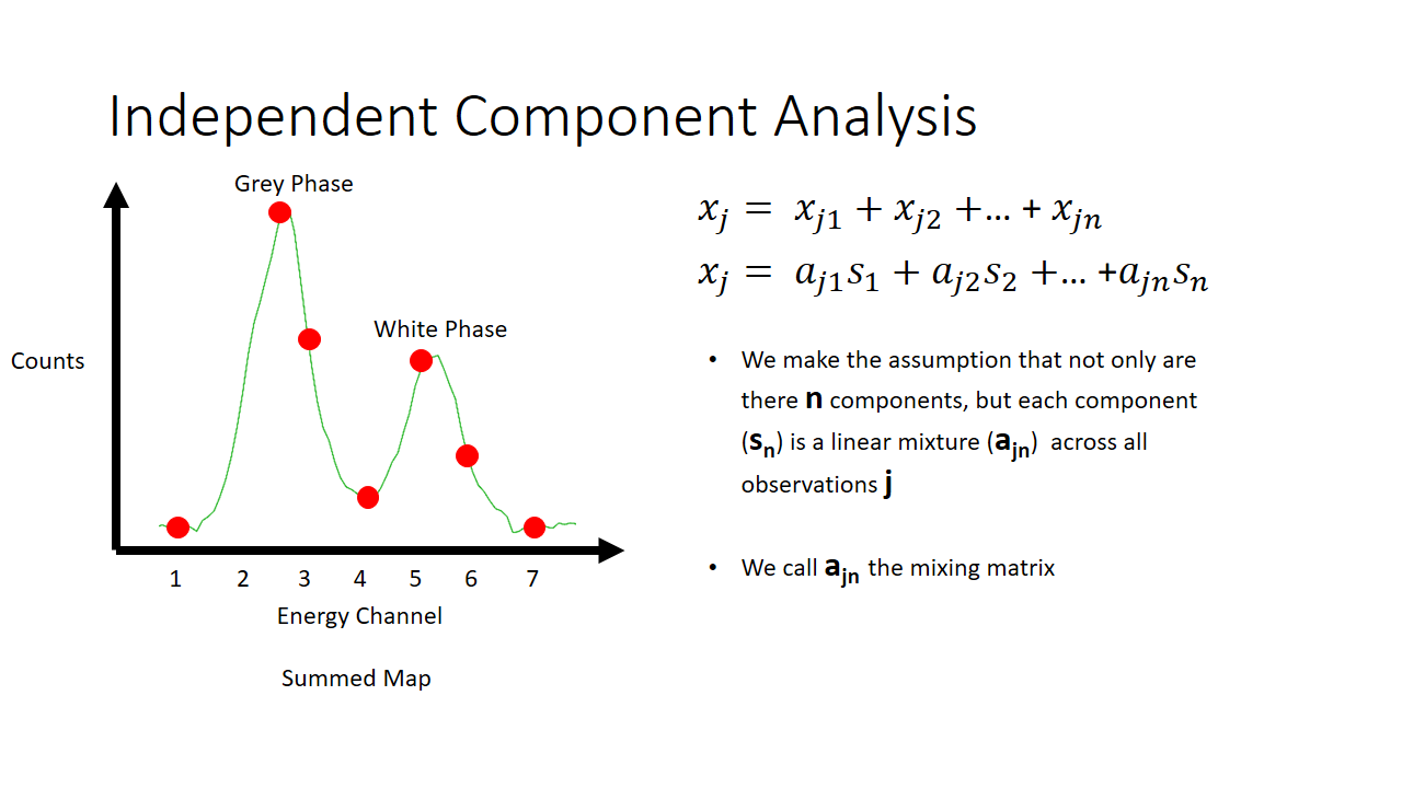
So now we have two major unknowns here. The mixing matrix a and the components s. We know what the mixture is like at every pixel, and we know that the components are not gaussian. In the case of our simple EELS spectra, we know there are two 7 variable components, and there are 2 linear factors for every observation.

In total then there are something like 40 variables that need to be solved for with only 16 observations. Quite a daunting task. This is made easier by knowing that the mixed signals have Gaussian character (via the Central Limit Theorem) so we seek to solve for the mixing matrix such that the applied transformation causes the extracted components to be maximally non-gaussian.

This can be solved numerically using a suite of algorithmic methods. I am not an expert in this field and I really cannot tell you how it works. This is about the extent of my knowledge here. I would defer the curious reader into reading about the FastICA method which is a commonly used approach to solve this problem.